
An updated overview of recent gradient descent algorithms
In this blog post, we will cover some of the recent advances in optimization for gradient descent algorithms. There are various sources online that compare the most famous approaches, such as the blogpost by Sebastian Ruder; this blogpost complements these exisiting overviews with more recent approaches, as well as extensive experiments.
Gradient descent algorithms are the optimizers of choice for training deep neural networks, and generally change the weights of a neural network by following the direction of the negative gradient of some loss function with respect to the weight. We are going to start off with the classic, and most popular, gradient descent algorithms, and move on towards more recent, and less known, algorithms. While the classic, age-old gradient descent algorithms remain the most popular, there are empirical and theoretical reasons to consider these newer alternatives.
For the rest of this blog, we will let \(\theta_{t}\) be the weights of the neural network at time step \(t\). \(g_t\) is the (usually, stochastic) gradient, which is the derivative of some loss \(\mathcal{L}(\theta_t)\) with respect to \(\theta_{t}\). The general idea of gradient descent is to minimize the loss \(\mathcal{L}(\theta_t)\) by walking in the direction of \(-g_t\).
For the most recent algorithms, jump to QHAdam.
Vanilla Gradient Descent
The story for modern day deep learning optimizers started with vanilla gradient descent. Vanilla gradient descent follows the below iteration with some learning rate parameter \(\eta\):
\[\theta_{t+1} = \theta_t - \eta \cdot g_t, \; \forall t,\]where the loss is the mean loss, calculated with some number of samples, drawn randomly from the entire training dataset. For Batch Gradient Descent (or simply Gradient Descent), the entire training dataset is used on each iteration to calculate the loss. For Stochastic Gradient Descent (SGD), one sample is drawn per iteration. In practice, generally a mini-batch is used, and common mini-batch sizes range from 64 to 2048. A mini-batch can significantly reduce the variance of the gradient without the large computation cost of using the entire dataset; the mini-batch gradient descent is so common that it is usually referred to as SGD. From now on, you can assume mini-batches are used for the computation of \(g_t\).
Momentum
Consider two cases, a) the local loss landscape is a smooth hill and b) the local loss landscape is a steep ravine. In the first case, the gradient descent algorithm may take a long time to reach the bottom of the hill, even though it is clearly traveling in the same direction. In the second case, the gradient descent algorithm may bounce back and forth between the walls of the steep ravine without reaching the bottom fast, and it would be great if the back and forth gradients could be averaged to reduce the variance.
These are the two common explanations for the need for a gradient accumulation or averaging mechanism, which leads us to momentum. Momentum is an exponential moving average of past gradients parameterized by \(\beta\) (commonly equal to 0.9), and is given by the below algorithm:
\[\theta_{t+1} = \theta_t + \eta v_{t}, \quad v_{t} = \beta v_{t-1} - g_t.\]This remains one of the two most popular optimizers for training deep neural networks1, and there is a long list of state-of-the-art results achieved using the momentum optimizer.
(There are various “vanilla” momentum implementations, that are seemingly different. However, most of them perform similarly, at the level of having small differences in the final solution. See also the blogpost by James Melville).
AdaGrad
AdaGrad (Adaptive Gradient) 2 is inspired by the intuition that weights, which are infrequently updated, should be updated with a larger learning rate than weights which are frequently updated. Basically, if a weight rarely gets a large gradient, it should make the most of it when it does receive a large gradient. This is realized by keeping a running additive sum of squared gradients per weight and dividing the learning rate by this running sum. Beginning with AdaGrad 2, the SGD recursion, per coordinate \(i\) of \(\theta\), becomes:
\[\theta_{t+1, i} = \theta_{t, i} - {\tfrac{\eta}{\sqrt{G_{t, ii} + \varepsilon}}} \cdot g_{t, i}, \quad \forall t,\]where \(G_t \in \mathbb{R}^{p \times p}\) is usually a diagonal preconditioning matrix as a summation of squares of past gradients, and \(\varepsilon > 0\) a small constant. Note the square root used on \(G_t\) - other powers between 0 and 1 can be used effectively too, but the square root is a good starting point.
This generally has two other implications: a) Less sensitive to hyperparameters than the momentum optimizer (some models can cost $100,000 to train once!), and b) this approximates the diagonal Hessian and is an approximation of a second order method using only first order information. These learning rate adaptive algorithms can be understood as utilizing current and past gradient information to design preconditioning matrices that better approximate the local curvature of the loss function.
RMSprop
However, the accumulation of squared gradients in AdaGrad can only increase, and this means if the optimizer is run for a sufficiently long time, in practice the subsequent updates are too small. RMSprop (Root Mean Squared Backpropagation) 3 substitutes the ever accumulating matrix \(G_t\) with a running average of squared gradients computed per iteration with discount factor \(\beta_2\) as: \(\mathcal{E}^{g \circ g}_{t+1} = \beta_2 \cdot \mathcal{E}^{g \circ g}_t + (1 - \beta_2) \cdot (g_t \circ g_t)\), where \(\beta_2\) was first proposed as 0.9 and a good default learning rate is 0.001. Here, \(\circ\) denotes the per-coordinate multiplication. Then, RMSprop updates as:
\[\theta_{t+1, i} = \theta_{t, i} - \tfrac{\eta}{\sqrt{\mathcal{E}^{g \circ g}_{t+1, i} + \varepsilon}} \cdot g_{t, i}, \quad \forall t.\]Adam
What if we add momentum to RMSprop? We arrive at Adam (Adaptive Momentum) 4. In addition to RMSprop, Adam keeps an exponentially decaying average of past gradients with discount factor \(\beta_1\): \(\mathcal{E}^{g}_{t+1} = \beta_1 \cdot \mathcal{E}^{g}_t + (1-\beta_1) \cdot g_t\), leading to the recursion:
\[\theta_{t+1, i} = \theta_{t, i} - \tfrac{\eta}{\sqrt{\mathcal{E}^{g \circ g}_{t+1, i} + \varepsilon}} \cdot {\mathcal{E}^g_{t+1, i}}, \quad \forall t,\]where usually \(\beta_1 = 0.9\) and \(\beta_2 = 0.999\), and a suggested learning rate 0.001. Observe that Adam is equivalent to RMSprop when \(\beta_1 = 0\). We mention again to note the square root for \(\mathcal{E}^{g \circ g}_{t+1, i}\), and that other powers between 0 and 1 have been used effectively (there is such an algorithm called Padam 5). Adam was first published in 2014, and remains the most popular adaptive learning rate algorithm till today. There have been, however, more effective adaptive algorithms since then, but adoption by the machine learning community has been slow.
AMSGrad
The motivation for AMSGrad 6 lay in the observation that Adam does not converge for a simple optimization problem. The authors resolve this issue with a technical detail in the proof of Adam related to the exponential moving average \(\mathcal{E}^{g \circ g}_{t}\). Instead of an exponential moving average, AMSGrad keeps a running maximum of \(\mathcal{E}^{g \circ g}\).
The AMSGrad algorithm is parameterized by learning rate \(\eta > 0\), discount factors \(\beta_1 < 1\) and \(\beta_2 < 1\), a small constant \(\epsilon\), and uses the update rule:
\[\hat{\mathcal{E}}^{g \circ g}_{t+1, i} = max(\hat{\mathcal{E}}^{g \circ g}_{t, i},\mathcal{E}^{g \circ g}_{t, i} ), \\ \theta_{t+1, i} = \theta_{t, i} - \tfrac{\eta}{\sqrt{\hat{\mathcal{E}}^{g \circ g}_{t+1, i} + \varepsilon}} \cdot {\mathcal{E}^g_{t+1, i}}, \quad \forall t,\]where \(\mathcal{E}^{g}_{t+1}\) and \(\mathcal{E}^{g \circ g}_{t+1}\) are defined identically to Adam. However, it is generally accepted that AMSGrad does not perform better than Adam in practice. Bonus: No one really knows what AMSGrad stands for.
AdamW
Weight decay is a technique in training neural networks which tries to keep the value of weights small. The intuition is large weights tend to overfit, and there needs to be a good reason for a weight to be large. This is usually implemented by adding a term to the loss function which is a function of the value of the weights, and this way a large weight will increase the total loss significantly. The most popular form of weight decay is L2 regularization, which penalizes the squared value of weights and is convenient for dealing with both positive and negative weights simultaneously and for differentiability. AdamW 7 modifies the typical implementation of weight decay regularization in Adam, by decoupling the weight decay from the gradient update. In particular, L2 regularization in Adam is usually implemented with the below modification where \(w_t\) is the rate of the weight decay at time t:
\[g_t = \nabla f(\theta_t) + w_t \theta_t ,\]while AdamW, instead, adjusts the weight decay term to appear in the gradient update:
\[\theta_{t+1, i} = \theta_{t, i} - \eta \Big( \tfrac{1}{\sqrt{\hat{\mathcal{E}}^{g \circ g}_{t+1, i} + \varepsilon}} \cdot {\mathcal{E}^g_{t+1, i}} + w_{t, i} \theta_{t, i} \Big), \quad \forall t.\]This turns out to make a difference in practice and has been adopted in parts of the machine learning community. You’d be surprised how some small details can make a noticeable difference in performance!
QHAdam
QHAdam (Quasi-Hyperbolic Adam) 8 is an adaptive learning rate extension of QHM (Quasi-Hyperbolic Momentum), introduced further below, to replace both momentum estimators in Adam with quasi-hyperbolic terms. Namely, QHAdam decouples the momentum term from the current gradient when updating the weights, and decouples the mean squared gradients term from the current squared gradient when updating the weights. In other words, it is a weighted average of the momentum and plain SGD, weighting the current gradient with an immediate discount factor \(\nu_1\), divided by a weighted average of the mean squared gradients and the current squared gradient, weighting the current squared gradient with an immediate discount factor \(\nu_2\). This quasi-hyperbolic formulation is capable of recovering Adam and NAdam 9, amongst others. Note that \(\mathcal{E}^{g}_{t+1}\) and \(\mathcal{E}^{g \circ g}_{t+1}\) below are defined identically to Adam. If that was confusing, take a look at the QHAdam algorithm below with the update rule:
\[\theta_{t+1, i} = \theta_{t, i} - \eta \Bigg[ \frac{(1 - \nu_1) \cdot g_t + \nu_1 \cdot \hat{\mathcal{E}}^{g}_{t+1}}{\sqrt{(1 - \nu_2) g_t^2 + \nu_2 \cdot \hat{\mathcal{E}}^{g \circ g}_{t+1}} + \epsilon} \Bigg], \quad \forall t,\]The hyperparameter choices for QHAdam are situational, and it is recommended \(\nu_2 = 1\) and setting \(\beta_2\) as in Adam are good starting points.
YellowFin
YellowFin 10 is a learning rate and momentum tuner motivated by robustness properties and analysis of quadratic objectives. For quadratic objectives, the optimizer tunes both the learning rate and the momentum to keep the hyperparameters within a region in which the convergence rate is a constant rate equal to the root momentum. This notion is extended empirically to non-convex objectives. On every iteration, YellowFin optimizes the hyperparameters to minimize a local quadratic optimization. For interested readers, we defer the many details to the paper. We note here that YellowFin with no tuning can be competitive with Adam and the momentum optimizer.
AggMo
Choosing the momentum parameter can be hard. The common choices of 0, 0.9, or 0.99 as the momentum parameter \(\beta\) can yield dramatically different performance and it is very difficult to predict the performance beforehand. If \(\beta\) is chosen too large for the task at hand, it can produce oscillating behavior and slow down convergence. On the other hand, if \(\beta\) is chosen too small for the task at hand, it can significantly increase training time and reduce performance. AggMo (Aggregated Momentum) 11 is an adaptive momentum algorithm and resolves this issue by taking a linear combination of multiple momentum buffers. It maintains \(K\) momentum buffers, each with a different discount factor, and averages them for the update. For the \(K\) momentum buffers, there are discount factors \(\beta \in \mathbb{R}^K\), and the overall update rule is:
\[({\mathcal{E}^{g}_{t+1}})^{(i)} = \beta^{(i)} \cdot ({\mathcal{E}^{g}_t})^{(i)} + g_t , \quad \forall i \in [1, K],\] \[\theta_{t+1, i} = \theta_{t, i} - \eta \Bigg[ \frac{1}{K} \cdot \sum_{i=1}^{K}{(\mathcal{E}^{g}_{t+1})^{(i)}} \Bigg], \quad \forall t.\]There is good empirical evidence that this reduces oscillations while maintaining acceleration on toy examples.
QHM
QHM (Quasi-Hyperbolic Momentum) 8 is another adaptive momentum algorithm which decouples the momentum term from the current gradient when updating the weights. In other words, it is a weighted average of the momentum and plain SGD, weighting the current gradient with an immediate discount factor \(\nu\). Note that this formulation is capable of recovering Nesterov Momentum 12, Synthesized Nesterov Variants 13, accSGD 14 and others. The QHM algorithm uses the update rule:
\[\mathcal{E}^{g}_{t+1} = \beta \cdot {\mathcal{E}^{g}_t} + (1 - \beta) \cdot g_t,\] \[\theta_{t+1, i} = \theta_{t, i} - \eta \Big[ (1 - \nu) \cdot g_t + \nu \cdot \mathcal{E}^{g}_{t+1} \Big], \quad \forall t.\]The authors recommend \(\nu = 0.7\) and \(\beta=0.999\) as a good starting point.
Demon
Demon (Decaying Momentum) 15 is a decaying momentum rule which is inspired by linear learning rate decay models which reduce the impact of a gradient to current and future updates. By decaying the momentum parameter, the total contribution of a gradient to all future updates is decayed. A particular gradient term \(g_{t}\) contributes a total of \(\eta \sum_{i} \beta^{i}\) of its ‘‘energy’’ to all future gradient updates, and this results in the geometric sum, \(\sum_{i = 1}^{\infty} \beta^{i} = \beta \sum_{i = 0}^{\infty} \beta^{i} = \beta/(1 - \beta)\). Decaying this sum results in the Demon algorithm. Let \(\beta_{\text{init}}\) be the initial \(\beta\); then at current step \(t\) with total \(T\) steps, the decay routine is given by solving the below for \(\beta_t\):
\[{\beta_t}/(1 - \beta_t) = (1 - {t}/{T}) \beta_{\text{init}}/(1 - \beta_{\text{init}}).\]Above, the fraction \((1 - t/T)\) refers to the proportion of iterations remaining. Note that Demon typically requires no hyperparameter tuning as it is usually decayed to 0 or a small negative value at time \(T\). Improved performance is observed by delaying the decaying. Demon can be applied to any gradient descent algorithm with a momentum parameter.
Experimental setup
We evaluated Adam, AMSGrad, AdamW, QHAdam, YellowFin, Demon Adam, Momentum (or referred to as SGD with Momentum (SGDM)), Aggmo QHM, and Demon SGDM, on six test problems. These include a variety of architectures - Residual CNNs, Non Residual CNNS, RNNs, generative models, and Capsule Networks - and datasets - CIFAR10, CIFAR100, STL10, PTB, MNIST, FMNIST. We generally perform a grid search over the learning rate and momentum. For the non-learning rate adaptive algorithms SGDM, Aggmo, and QHM, we decay the learning rate by 0.1 at 50% and 75% of the total epochs, following the standard in the literature.
We describe the six test problems in this blog.
- CIFAR10 - ResNet18 CIFAR10 contains 60,000 32x32x3 images with a 50,000 training set, 10,000 test set split. There are 10 classes. ResNet18 16 is an 18 layers deep CNN with skip connections for image classification. Trained with a batch size of 128.
- CIFAR100 - VGG16 CIFAR100 is a fine-grained version of CIFAR-10 and contains 60,000 32x32x3 images with a 50,000 training set, 10,000 test set split. There are 100 classes. VGG16 17 is a 16 layers deep CNN with extensive use of 3x3 convolutional filters. Trained with a batch size of 128
- STL10 - Wide ResNet 16-8 STL10 contains 1300 96x96x3 images with a 500 training set, 800 test set split. There are 10 classes. Wide ResNet 16-8 18 is a 16 layers deep ResNet which is 8 times wider. Trained with a batch size of 64.
- FMNIST - CAPS MNIST contains 60,000 32x32x1 grayscale images with a 50,000 training set, 10,000 test set split. There are 10 classes of 10 clothing items. Capsule Networks 19 represent Neural Networks as a set of capsules, where each capsule encodes a specific entity or meaning. The activations of capsules depend on comparing incoming pose predictions, as opposed to standard neural networks. The Capsule Network uses 3 iterations in the routing algorithm. Trained with a batch size of 128.
- PTB - LSTM PTB is an English text corpus containing 929,000 training words, 73,000 validation words, and 82,000 test words. There are 10,000 words in the vocabulary. The model is stacked LSTMs 20 with 2 layers, 650 units per layer, and dropout of 0.5. Trained with a batch size of 20.
- MNIST - VAE MNIST contains 60,000 32x32x1 grayscale images with a 50,000 training set, 10,000 test set split. There are 10 classes of 10 digits. VAE 21 with three dense encoding layers and three dense decoding layers with a latent space of size 2. Trained with a batch size of 100.
Results
For clarity, the algorithms are separated into adaptive learning rate (Adam, AMSGrad, AdamW, QHAdam, Demon Adam) and non-adaptive learning rate (SGDM, AggMo, QHM, Demon SGDM). We run a variety of epochs to demonstrate the performance of optimizers under different runtimes.
Adaptive learning rate algorithms
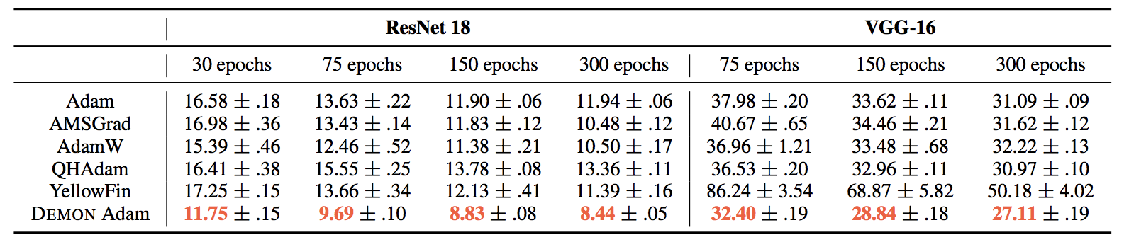
We first consider the CIFAR10 - ResNet18 and CIFAR100 - VGG16 settings below. Although Adam is the most popular adaptive learning rate algorithm, it is clear in these two classic image classification settings Adam does not perform the best. Holistically, Adam is a relatively middling algorithm, although this is a remarkable observation in itself since it has been 6 years (!) since its inception. YellowFin’s performance was not substantially improved through hyperparameter tuning, and it is remarkably competitive with the other state-of-the-art algorithms. Demon Adam is clearly the best performing algorithm and is the only algorithm to achieve state-of-the-art performance compared to momentum methods on these two settings.
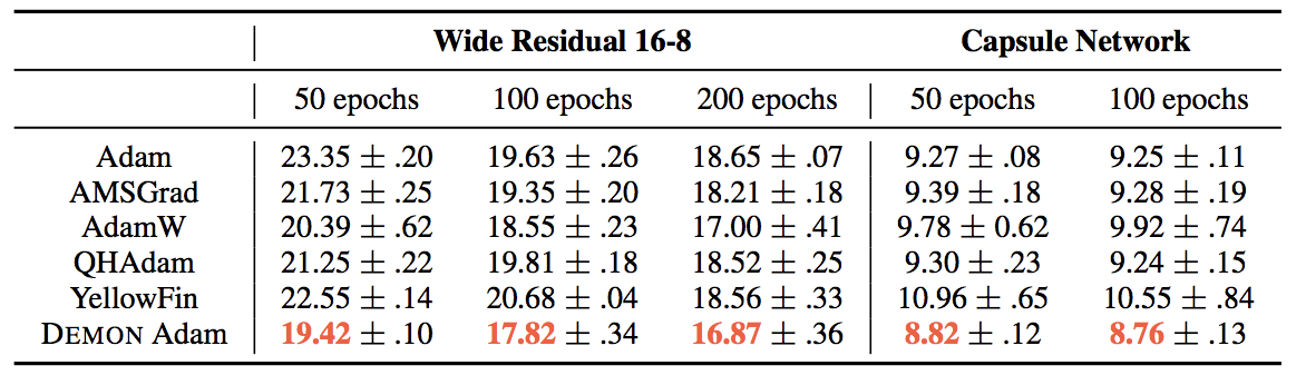
Next, we present the STL10 - Wide ResNet 16-8 and FMNIST - CAPS settings below. AdamW performs particularly strong in the Wide ResNet setting, with almost a 1.5% generalization error gap with the other algorithms. In the same setting, YellowFin actually outperforms Adam, although it does not perform as well on the Capsule Networks. We once again see Demon Adam as the best performing algorithm, and the only algorithm which is competitive with state-of-the-art results.
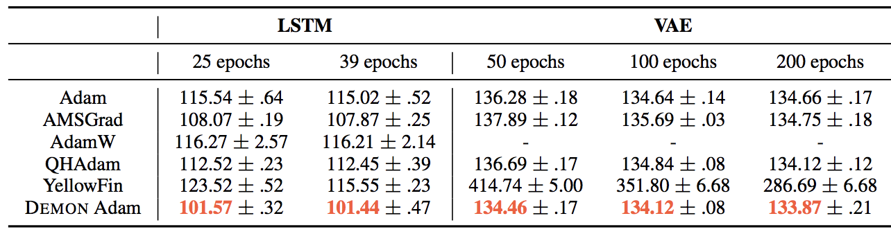
We move on to language models and generative models with PTB - LSTM and MNIST - VAE. The LSTM results are not particularly interesting - none of the algorithms come close to being competitive with the momentum optimizers. For MNIST - VAE, due to the vanilla VAE used here without weight decay, AdamW is unsuitable for comparison. Here, we see the lead for Demon Adam shrink for larger epochs. YellowFin fails to find a good result.
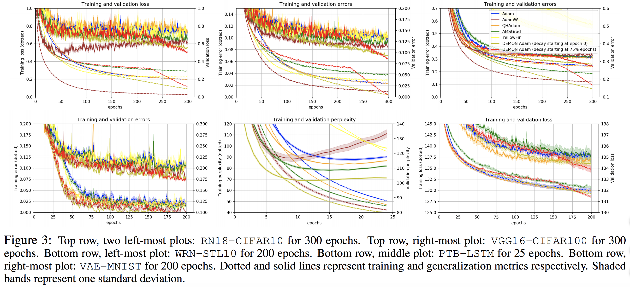
We plot the results below. In general, Demon Adam outperforms the other algorithms and continues to learn after they have plateaued. Notice also the overall improved performance of AdamW over Adam.
Non-adaptive learning rate algorithms
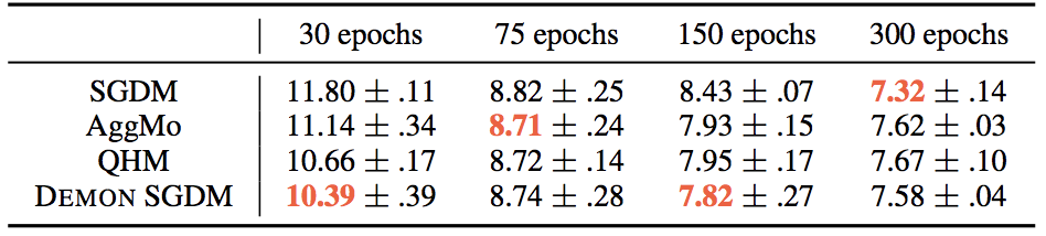
We first present results on CIFAR10 - ResNet18. Note that we apply learning rate decay by 0.1 to SGDM, AggMo and QHM at 50% and 75% of the total epochs. For a small number of epochs, Demon SGDM is a strong performer, notably without the need to tune learning rate decay. However, for any reasonable number of epochs all the algorithms essentially equalize. In other words, SGDM holds its own here.
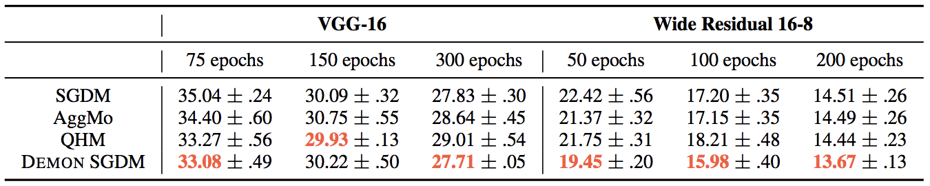
Moving on to CIFAR100 - VGG16 and STL10 - Wide ResNet, this is where Demon SGDM really shines. Demon SGDM produces state-of-the-art performance for VGG16, and is almost 1% better for Wide ResNet. At the same time, it is worth noting the strong performance of SGDM relative to AggMo and QHM. Not so bad for an age-old algorithm!
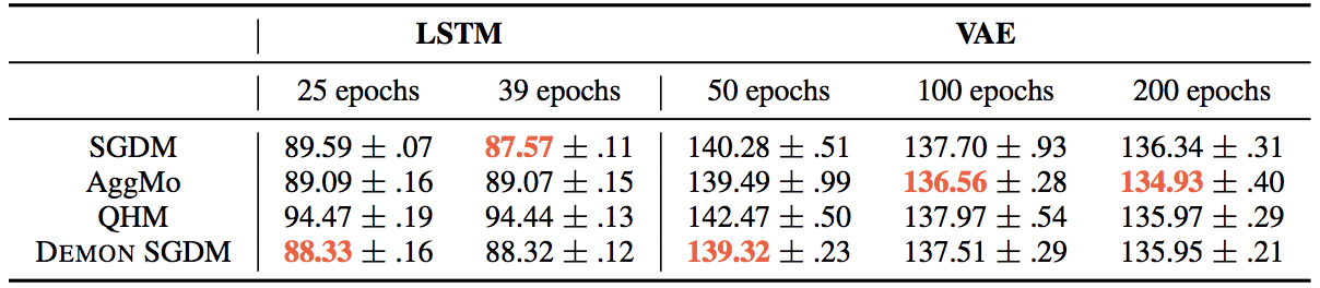
Turning to PTB - LSTM, SGDM, or Demon SGDM, is again the optimizer of choice. However, the language modeling task deserves some more investigation as there more modern models out there. In terms of learning rate decay, this is also trickier as the model can overfit if trained for too long. For MNIST - VAE, Demon SGDM performs well, and AggMo achieves the best generalization loss here for large number of epochs by 1%.
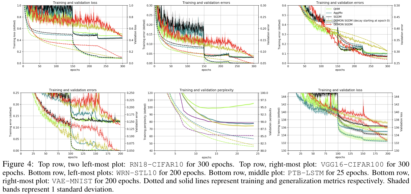
Results are plotted below. In the grand scheme of things, learning rate decay seems to equalize many of the algorithms. SGDM remains a very, if not the most, effective algorithm. Demon SGDM with decay delayed till 75% of epochs performs well too, and appears to be an alternative to, and in many cases better than, learning rate decay.
What to use?
If you have no budget for hyperparameter tuning at all, then YellowFin is a good choice due to its decent empirical performance where it self-tunes both the learning rate and the momentum parameters.
With some budget for hyperparameter tuning, you can consider the adaptive learning rate algorithms, namely the more recent AdamW or QHAdam, in addition to Demon which appears to give a substantial boost too.
Lastly, if getting the best performance is your utmost concern, SGDM is probably still the algorithm of choice, perhaps with Demon. It may also be worth giving QHM or AggMo a shot.
Of course, these recommendations are domain specific - there are some domains where adaptive learning rate algorithms outperform standard momentum algorithms.
Conclusion
We hope this blog has been helpful in shedding light on the recent optimization algorithms for training deep neural networks. We apologize if we missed any algorithms - there are a lot of choices out there! Let us know what we missed and what works for you!
-
Goodfellow, I., Bengio, Y., Courville, A., and Bengio, Y. Deep learning, volume 1. MIT Press, 2016. ↩︎
-
Duchi, J., Hazan, E., and Singer, Y. Adaptive subgradient methods for online learning and stochastic optimization. Journal of Machine Learning Research, 12(Jul):2121– 2159, 2011. ↩︎ ↩︎2
-
Hinton, G., Srivastava, N., and Swersky, K. Neural networks for machine learning lecture 6a overview of minibatch gradient descent. Cited on, 14:8, 2012. ↩︎
-
Kingma, D. P. and Ba, J. Adam: A method for stochastic optimization. arXiv preprint arXiv:1412.6980, 2014. ↩︎
-
Chen, J. Chen and Gu, Q. Closing the generalization gap of adaptive gradient methods in training deep neural networks. arXiv preprint arXiv:1806.06763, 2018. ↩︎
-
Reddi, S. J., Kale, S., and Kumar, S. On the convergence of Adam and beyond. arXiv preprint arXiv:1904.09237, 2018. ↩︎
-
Loshchilov, I. and Hutter, F. Fixing weight decay regularization in adam. arXiv preprint arXiv:1711.05101, 2017. ↩︎
-
Ma, J. and Yarats, D. Quasi-hyperbolic momentum and Adam for deep learning. arXiv preprint arXiv:1810.06801, 2018. ↩︎ ↩︎2
-
Dozat, T. Incorporating nesterov momentum into adam. ICLR Workshop, (1):20132016, 2016. ↩︎
-
Zhang, J. and Mitliagkas, I. Yellowfin and the art of momentum tuning. arXiv preprint arXiv:1706.03471, 2017. ↩︎
-
Lucas, J., Sun, S., Zemel, R., and Grosse, R. Aggregated momentum: Stability through passive damping. arXiv preprint arXiv:1804.00325, 2018. ↩︎
-
Nesterov, Y. A method for solving the convex programming problem with convergence rate of (1/k2). Soviet Mathematics Doklady, 27(2):372–376, 1983 ↩︎
-
Lessard, L., Recht, B., and Packard, A. Analysis and design of optimization algorithms via integral quadratic constraints. SIAM Journal on Optimization, 26(1):57–95, 2016. ↩︎
-
Jain, P., Kakade, S. M., Kidambi, R., Netrapalli, P., and Sidford, A. Accelerating stochastic gradient descent for least squares regression. arXiv preprint arXiv:1704.08227, 2017. ↩︎
-
Chen, J., Kyrillidis, A. Decaying Momentum Helps Neural Network Training. arXiv preprint arXiv:1910.04952, 2019. ↩︎
-
He, K., Zhang, X., Ren, S., and Sun, J. Deep residual learning for image recognition. In Proceedings of the IEEE conference on computer vision and pattern recognition, pp. 770–778, 2016 ↩︎
-
Simonyan, K. and Zisserman, A. Very deep convolutional networks for large-scale image recognition. arXiv preprint arXiv:1409.1556, 2014. ↩︎
-
Zagoruyko, S. and Komodakis, N. Wide residual networks. arXiv preprint arXiv:1605.07146, 2016. ↩︎
-
Sabour, S., Fross, N., and Hinton, G. Dynamic routing between capsules. In Advances in neural information processing systems, 2017. ↩︎
-
Hochreiter, S. and Schmidhuber, J. Long short-term memory. Neural computation, 9(8):1735–1780, 1997. ↩︎
-
Kingma, D. P. and Welling, M. Auto-encoding variational bayes. arXiv preprint arXiv:1312.6114, 2015. ↩︎